How to use the map-so-ii function? • so.ii

Introduction

This vignette demonstrates the use of the map_so_ii function from the so.ii package for creating thematic maps of spatial data within the geographical perimeter of the so-ii observatory. The function provides a flexible way to visualize various datasets, including catchments, collectivities, hydrographic networks, and more. This document will cover the available options and demonstrate how to customize the resulting plots.

Basic Usage

The map_so_ii function takes a spatial object (e.g., an sf object) as input and generates a thematic map based on the specified options. Here’s a simple example:

library(sf)
library(so.ii)

# Create a sample spatial object 
data = st_as_sf(
  data.frame(x = c(3.7, 3.8, 4.0), y = c(43.6, 43.7, 43.65)), 
  coords = c("x", "y")
)

# Generate a basic map
map_so_ii(dataset = data, pch = 19, col = "red")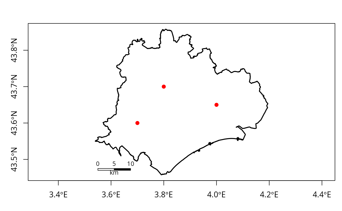

If you wish to add a legend to your plot, just use a list with the elements to be passed to the base plot legend() function. Here is an example:

map_so_ii(
  dataset = data, pch = 19, col = "red",
  dataset_legend = list(
    x = "bottomright",
    legend = "random points",
    col = "red",
    pch = 19
  )
)

Theme Specification

The theme argument controls the overall appearance of the map. Here are the available themes:

none: Displays only the perimeter of the spatial object.
catchment: Visualizes catchment areas, with a detail level ranging from 1 to 3.
catnat: Displays information on “Arrêtés Cat Nat” (natural disaster decrees) at the collectivity scale.
clc: Visualizes the CORINE Land Cover (CLC) dataset.
hydro: Displays the hydrographic network, with different detail levels (rivers, canals, water bodies).
onrn: Displays data from the “Observatoire National des Risques Naturels” (ONRN) at the collectivity scale.
osm: Uses a tile from OpenStreetMap as a background.
population: Displays population data at the collectivity scale.

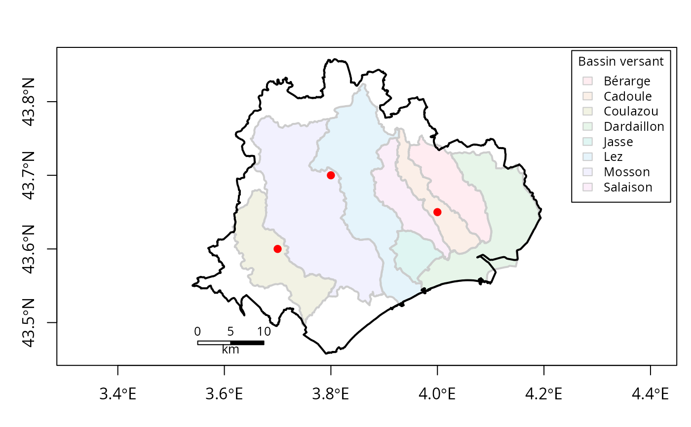
Here’s an example of creating a map with the catchment theme:

map_so_ii(
  dataset = data, pch = 19, col = "red", 
  theme = "catchment", 
  detail = "2"
)

Theme legends are also available. Here is the same example displaying the legend associated:

map_so_ii(
  dataset = data, pch = 19, col = "red", 
  theme = "catchment", 
  detail = "2",
  theme_legend = TRUE
)

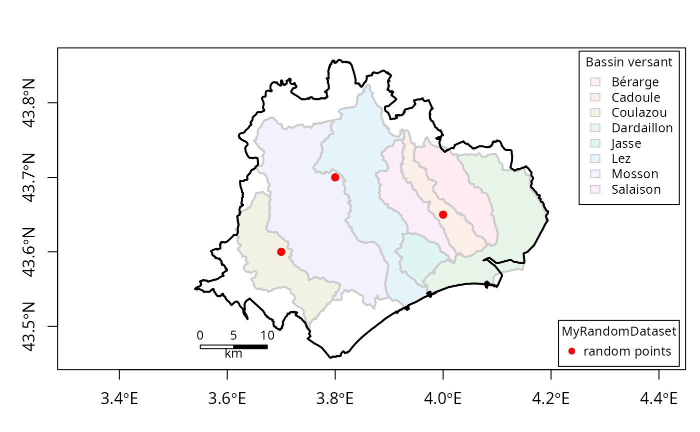
You can combine theme legends and your own legend as follows:

map_so_ii(
  dataset = data, pch = 19, col = "red",
  dataset_legend = list(
    x = "bottomright",
    legend = "random points",
    col = "red",
    pch = 19,
    title = "MyRandomDataset"
  ), 
  theme = "catchment", 
  detail = "2",
  theme_legend = TRUE
)

Detail Specification

The detail argument allows you to customize the appearance of certain themes. The available detail levels depend on the chosen theme. Here’s a breakdown:

catchment: detail can be “none”, “1”, “2”, or “3”, controlling the level of detail in the catchment visualization.
catnat: detail can be “inondation”, “submersion”, or “nappe”, specifying the type of natural disaster to visualize.
clc: detail can be “so.ii”, “crop”, or “both”, determining which CLC categories to display.
collectivity: detail can be “none”, “syble”, “symbo”, “epci”, or “syndicate”, controlling the type of collectivity boundaries to display.
hydro: detail can be “none”, “1”, “2”, “3”, or specific types like “canal”, “river”, “waterbody”.

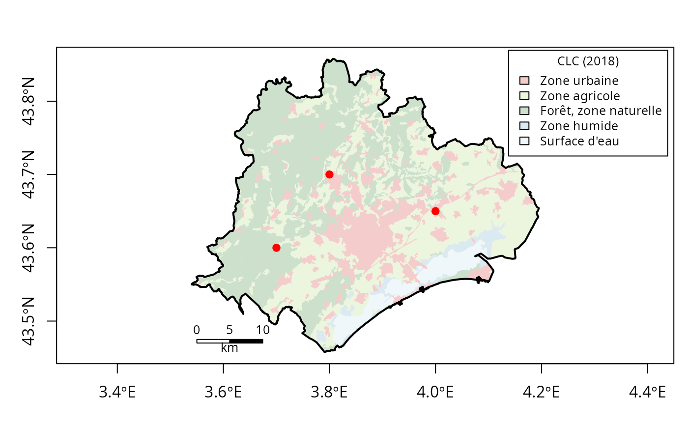
For example, to display the CLC dataset with only information inside the so.ii limit:

map_so_ii(
  dataset = data, pch = 19, col = "red", 
  theme = "clc", 
  detail = "so.ii",
  theme_legend = TRUE
)

Year Specification

The year argument allows you to specify the year for certain themes, such as population or onrn. If no year is specified, the latest available year will be used. For themes that support multiple years, you can provide a vector of years to visualize changes over time.

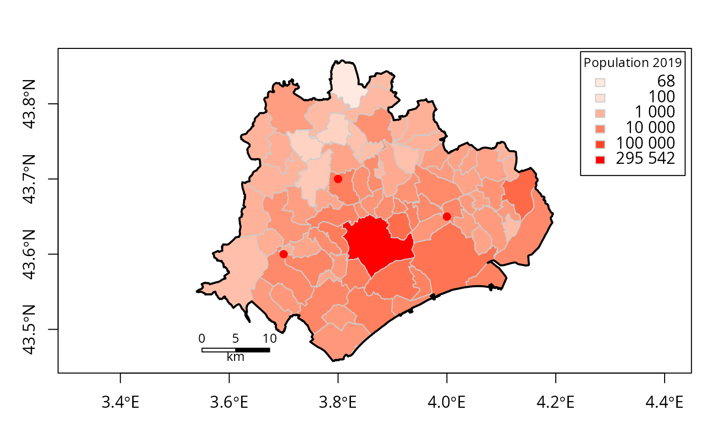
Single year

map_so_ii(
  dataset = data, pch = 19, col = "red", 
  theme = "population", 
  year = "2019",
  theme_legend = TRUE
)

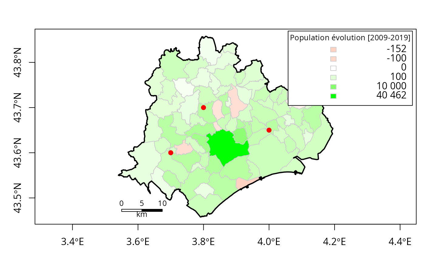
Multiple years

map_so_ii(
  dataset = data, pch = 19, col = "red", 
  theme = "population", 
  year = c("2009", "2019"),
  theme_legend = TRUE
)

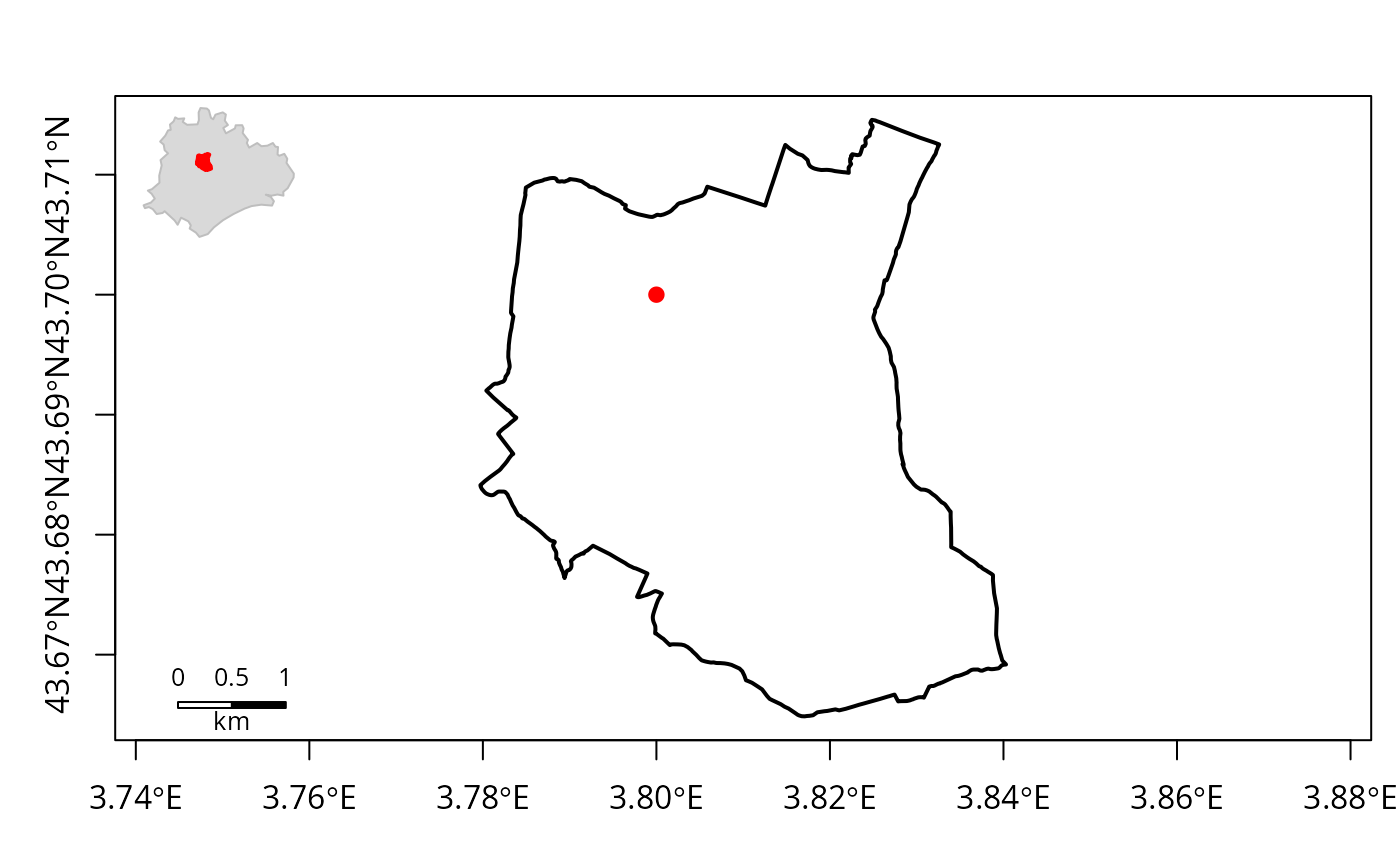
Scope Specification

The scope argument defines the spatial extent of the map. By default, it uses the entire extent of the input dataset. You can also specify a specific spatial object (e.g., an sf object) to limit the map to a particular area.

map_so_ii(
  dataset = data, pch = 19, col = "red", 
  scope = "34255",
  inset = "so-ii",
)

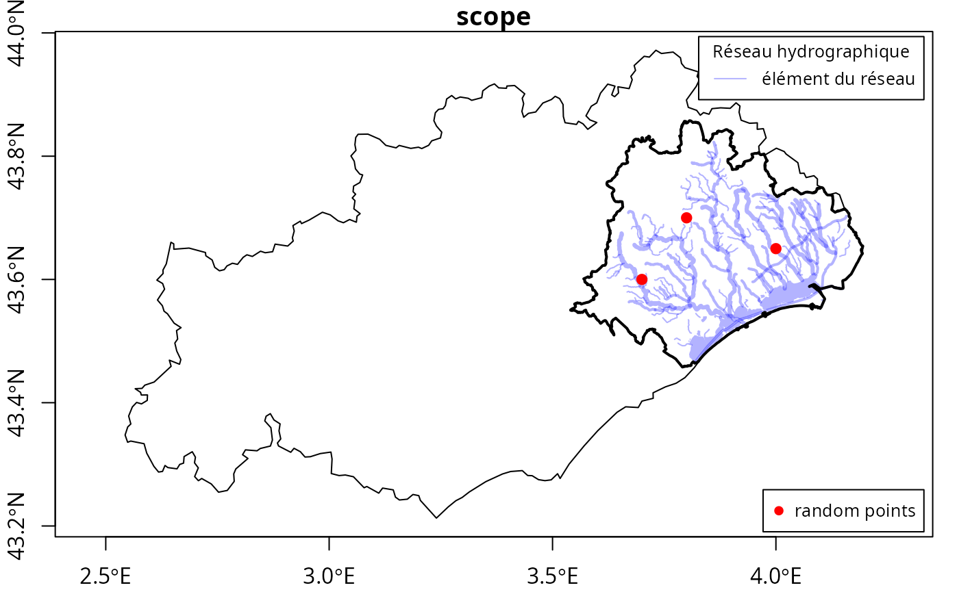
Advanced Options

The map_so_ii function also offers several other options for customization:

add: A logical value indicating whether to add the plot to an existing plot.

plot(
  so_ii_inset[so_ii_inset$scope == "Hérault",], 
  col = "white", 
  axes = TRUE, 
  reset = FALSE
)
map_so_ii(
  dataset = data, pch = 19, col = "red",
  dataset_legend = list(
    x = "bottomright",
    legend = "random points",
    col = "red",
    pch = 19
  ), 
  theme = "hydro",
  theme_legend = TRUE,
  add = TRUE
)

path: A character string specifying the file path to save the plot. The file extension determines the graphics device to use (e.g., “pdf”, “png”, “jpg”, “svg”).