#> Loading required package: floodam.building
library(floodam.building)

# set up model to use example shipped with floodam
model_path = list(
  data = system.file("extdata", package = "floodam.building"),
  output = tempdir()
)Simulating the hydraulic behavior of the interior of a building
The function analyse_model() of floodam.building is great to estimate flood damage functions for events lasting up to or longer than 48 hours. As is standard practice, flood damage functions generated with the function analyse_model() do not take into account the hydraulic dynamics inside your building. However, accounting for these dynamics in flash flood events can be of the utmost importance.
Fortunately floodam.building has an additional function, analyse_hydraulic(), which simulates the hydraulics inside your building for a specified flood scenario (provided by the generate_limnigraph() function). This function allows you to estimate, among other things, the actual floodwater depth inside your building, improving the precision of damage estimation for short events.
Set up
This vignette is going to help you simulate the hydraulic behavior of the interior of a building using floodam.building. To do so, you need 2 key inputs:
- A model: Contains the geometric and hydraulic description of the building. It defines rooms, walls, openings, and their connections, as well as elevation data and damage functions.
- A limnigraph: The evolution of the floodwater depth in front of each external wall exposed to the flood as well as the initial floodwater depth in the interior of the building (usually 0).
The library floodam.building provides methods to calculate each of these elements. Let us see how it works using one of the models shipped with floodam.building as an example. The models are available in your library’s installation folder. To make them available, just ask R to locate them:
We are going to use the model called adu_t. This model proposes a 4-room house where three of them are organized around a central living room (see below). To determine the two first key inputs, the function analyse_model() provides you with the stage hydraulic. Let us call the analyse_model() function to create the object model, using the shipped adu_t model and specifying c("load", "extract", "hydraulic") as stages of analysis. This model contains multiple type of informations relevant to our hydraulic modeling: the surface and floor level of each room, the connections between two rooms as well as the connections with the exterior of the buildings. Hereafter we will refer to these connections as exchanges.
model = analyse_model(
  model = "adu_t",
  type = "adu",
  stage = c("load", "extract", "hydraulic"),
  path = model_path,
  verbose = FALSE
)
plot(model)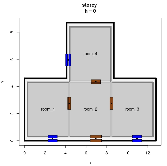
The object model includes several slots. The slot called hydraulic contains four different slots, each of which contains a data.frame:
exchanges_openexchanges_closeexchanges_combinerooms
The data.frame in the slot rooms corresponds to the first key inputs, while the data.frames in the slots exchanges_open, exchanges_close and exchanges_combine are variants of the second key input: all openings open, all openings closed but not waterproof, and all exterior openings closed and all interior openings open, respectively. Below you can see the examples for the data.frames in the slots rooms (right) and exchanges_close (left).
| exchange | width | H_abs | height | x | y | discharge_coeff | |
|---|---|---|---|---|---|---|---|
| 1 | door1|room_2 | 1.1 | 0.0 | 0.005 | 6.95 | 0.15 | 0.42 |
| 2 | window1|room_1 | 0.9 | 0.9 | 0.005 | 2.75 | 0.15 | 0.42 |
| 3 | window2|room_3 | 0.9 | 0.9 | 0.005 | 10.95 | 0.15 | 0.42 |
| 4 | window3|room_4 | 0.9 | 0.9 | 0.005 | 4.25 | 5.95 | 0.42 |
| 6 | room_1|room_2 | 0.9 | 0.0 | 0.005 | 4.35 | 2.75 | 0.42 |
| 8 | room_2|room_3 | 0.9 | 0.0 | 0.005 | 8.45 | 2.75 | 0.42 |
| 9 | room_2|room_4 | 0.9 | 0.0 | 0.005 | 6.95 | 4.35 | 0.42 |
| room | surface | H_abs | initial_depth |
|---|---|---|---|
| room_1 | 16 | 0 | 0 |
| room_2 | 16 | 0 | 0 |
| room_3 | 16 | 0 | 0 |
| room_4 | 16 | 0 | 0 |
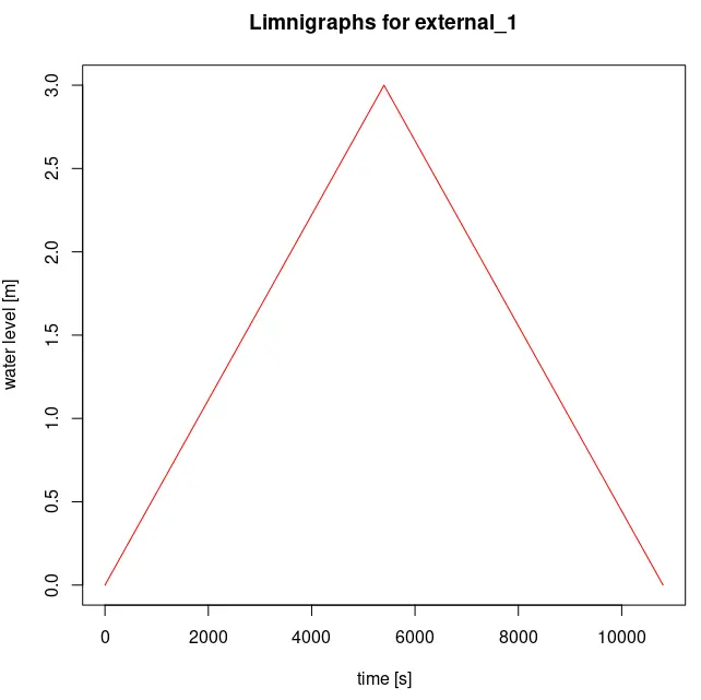
To simulate the third key input, floodam.building provides the function generate_limnigraph(). This function generates a limnigraph, i.e. the evolution of floodwater depth against time. This limnigraph is meant to represent the evolution of floodwater depth outside the building during the flood event. You need to manually provide different parameters to this function:
-
model: the output of the functionanalyse_model()(see above) -
time: vector of time steps in seconds. Usually it contains three elements: the initial time step, the time step where water outside the building is at its peak, and the final time step. In the example provided this time steps are 0, 5400 and 10800 seconds. -
depth: vector of floodwater depth in meters. This vector contains as many elements as the vector of time steps. It indicated the water depth in each time step. -
exposition: external walls that are exposed to the flood event. In the example provided, all the external walls are assumed to be exposed to this particular flood event.
The generate_limnigraph() function returns a list with two slots: the first one, named limnigraph, containing a matrix named with the time steps as rows and the external walls as columns, and the second one, named exposition, with the exposition of external walls.
Warning Depth and exposition parameters need to have the same facade names and they need to be named with the word facade in it.
Simulate hydraulics
Once the two key parameters are determined, the simulation of the building’s hydraulic dynamics during the flood event designed can be simulated using the function analyse_hydraulic(). To use this functions you should provide, at least, the following four parameters:
-
model: the output of the functionanalyse_model()(see above) -
limnigraph: the output of the functiongenerate_limnigraph()(see above) -
stage: what you want the function to perform: hydraulic, damaging, dangerosity, graph, save, display -
opening_scenario: one of the following options: open, close, combine
The function analyse_hydraulic() can be provided with several more parameters. Please check its documentation to learn more
hydraulic = analyse_hydraulic(
  model = model,
  limnigraph = flood,
  opening_scenario = "close",
  stage = c("hydraulic"),
  sim_id = "integrated_model"
)
Well done! You have now successfully processed your first hydraulic analysis. It is available inside the object hydraulic. This object is an object of the class hydraulic. Let us explore it further.
The object hydraulic that we have created contains five slots, each of them containing a matrix:
- The evolution of floodwater depth in each room
h(m). - The evolution of floodwater depth in each room compared to the ground level
z(m). - The evolution of the water flow through each opening
eQ(m³/s). - The evolution of the flow section through each opening
eS(m²). - The evolution of the flow velocity (calculated with the volume and section data) through each opening
ve(m/s). - The evolution of the water volume in each room
vo(m³). - The maximum floodwater depth in each room and their time stamp
hmax(m).
Let us explore the slot h. The matrix in this slot contains a column showing the time evolution (in seconds), a column per room in your building plus another column for the exposed external walls showing the evolution of the floodwater depth (in meters). Below you can see a table with its ten first lines.
| time | room_1 | room_2 | room_3 | room_4 | facade_1 |
|---|---|---|---|---|---|
| 0.0 | 0 | 0.0e+00 | 0 | 0 | 0.0000000 |
| 0.5 | 0 | 1.0e-07 | 0 | 0 | 0.0001389 |
| 1.0 | 0 | 3.0e-07 | 0 | 0 | 0.0002778 |
| 1.5 | 0 | 5.0e-07 | 0 | 0 | 0.0004167 |
| 2.0 | 0 | 9.0e-07 | 0 | 0 | 0.0005556 |
| 2.5 | 0 | 1.5e-06 | 0 | 0 | 0.0006944 |
| 3.0 | 0 | 2.3e-06 | 0 | 0 | 0.0008333 |
| 3.5 | 0 | 3.3e-06 | 0 | 0 | 0.0009722 |
| 4.0 | 0 | 4.5e-06 | 0 | 0 | 0.0011111 |
| 4.5 | 0 | 5.9e-06 | 0 | 0 | 0.0012500 |
In the table above we can see that the water rises in a linear fashion for facade_1. The entrance door (door_1 in the model) connects the exterior and the interior of the house through the room_2. Since this door is closed but not waterproof, water is flowing directly to the room_2 through the clearance. The rest of the rooms are connected to the room_2 though their respective doors, so they all fill with water as well but at a slower rate (the table above shows 0 as value because knitr::kable()’s precision is not high enough to display numbers lower than 10E-8).
Basic visualization
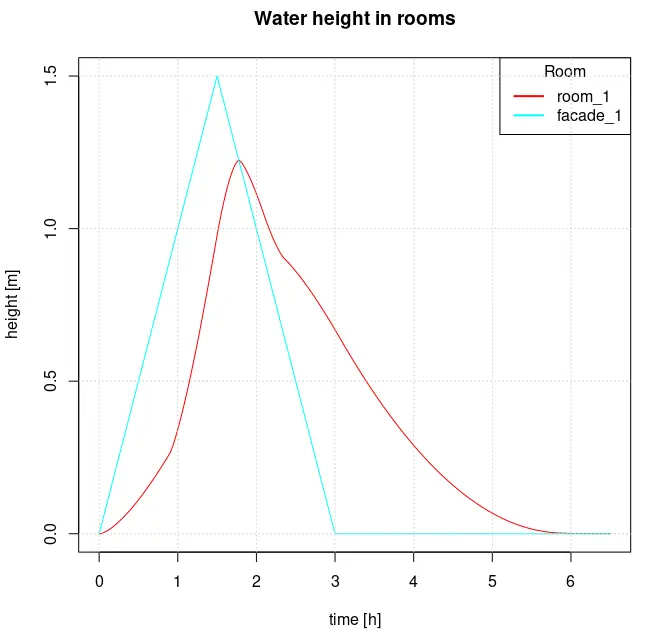
Methods to visualize key information stored in objects of class hydraulic have been implemented in floodam.building. By default, if you plot the hydraulic object, you will obtain the evolution of water height (in meters) for each room, using the elevation of each room as the reference.
#> visualization of the floodwater depth
plot(hydraulic)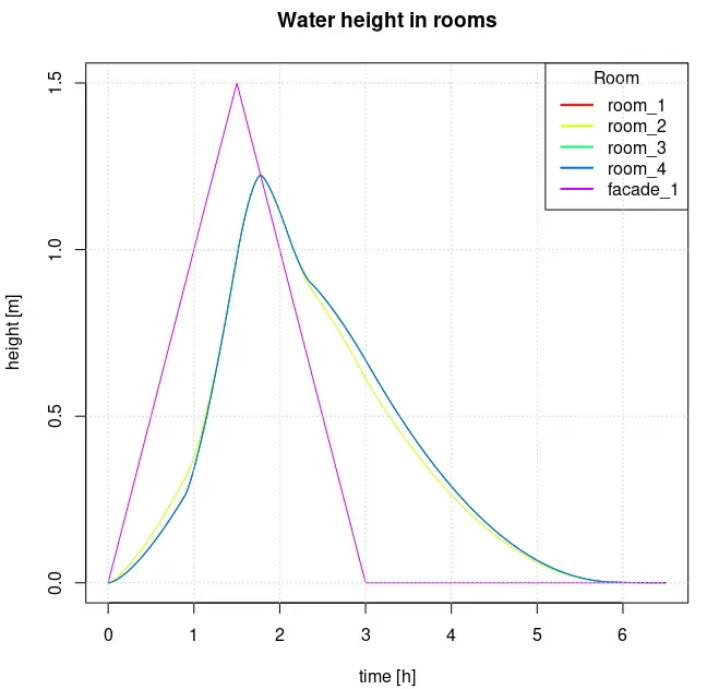
You can see that water depth is identical for room_1 room_3 room_4 due to the symmetry of the building. You can also control the data displayed by using the parameter view in your call to the plot() function. The code above is the equivalent of providing the parameter view with the value height. Alternatively, you can add the value display to the stages provided in your call to the analyse_hydraulic() function.
#> visualization of the floodwater depth
plot(hydraulic, view = "height")
There are two other values that you can use for this parameter:
-
level: to obtain a visualization of the evolution of the water height (in meters) for each room, using the elevation of the building as reference. In this case the render would be the same as
view = heightas all the rooms are on the same elevation: 0m.
#> visualization of the floodwater discharge in the openings
plot(hydraulic, view = "level")- discharge: to obtain the visualization of the evolution of the discharge (m³/s) for each opening.
#> visualization of the floodwater discharge in the openings
plot(hydraulic, view = "discharge")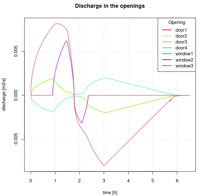
It is worth noting that openings are oriented, therefore you can notice either symmetry or superposition for door_2 door_4 door_3, again due to the symmetry of the building. If you need to know which openings are connecting the rooms you can look at this data.frame.
| room | name |
|---|---|
| external | door1 |
| external | window1 |
| external | window2 |
| external | window3 |
| room_1 | window1 |
| room_1 | door4 |
| room_2 | door1 |
| room_2 | door2 |
| room_2 | door3 |
| room_2 | door4 |
When working with larger buildings the graphs can start to be messy and overloaded. To clear it up you can select only certain rooms or openings by using the parameter selection.
If you wish to save the visualizations, you can use the device and output_path parameters in the function plot(). You can either save visualizations in PNG or PDF formats.
#> visualization of the floodwater discharge in the openings
plot(hydraulic, view = "height", device = "pdf", output_path = model[["path"]][["model_output_hydraulic"]])
Saving
Since floodam.building can be used as a virtual laboratory, we have implemented procedures to help you run experimental designs. For instance, you can use the parameter sim_id when calling the analyse_hydraulic() function in order to properly identify the simulation/s in your experimental design. You can also provide the values graph and/or save to the stages in the call to the analyse_hydraulic() function. The parameter what allows you to select what outputs you want to save.
hydraulic = analyse_hydraulic(
  model = model,
  limnigraph = flood,
  opening_scenario = "close",
  stage = c("hydraulic", "graph", "save"),
  what = c("h", "eQ"),
  sim_id = "integrated_model"
)
The value graph saves in the temporary folder the basic visualisation of water height and discharge in PNG format. The value save works in combination with the paramater what, allowing the user to store in the temporary folder the matrices provided to the what parameter as .csv.gz compressed files.
Get damages
If you’ve come to floodam.building it’s for a good reason, and you are probably interested in estimating damages. Here we are! In this part we’ll see how to estimate damages using the hydraulic dynamics you have just simulated. To do so, simply rerun the function analyse_hydraulic() adding the value damaging to the stages.
hydraulic = analyse_hydraulic(
  model = model,
  limnigraph = flood,
  opening_scenario = "close",
  stage = c("hydraulic", "damaging")
)
And here you go, the object hydraulic now contains a new slot named damage with a matrix showing the damage estimated with the highest floodwater depth reached in each room and outside (for the exposed external walls).
hydraulic[["damage"]] |> knitr::kable()| room_1 | room_2 | room_3 | room_4 | facade_1 | total | |
|---|---|---|---|---|---|---|
| damage | 3064.803 | 1491.884 | 3264.803 | 6414.803 | 4378.75 | 18615.04 |
For a more in-depth guide on how to build your own damage function with the hydraulic behavior taken in account you can read this guide here.
That’s all for the stages, if you want to run all of them at once just use stage = "all".
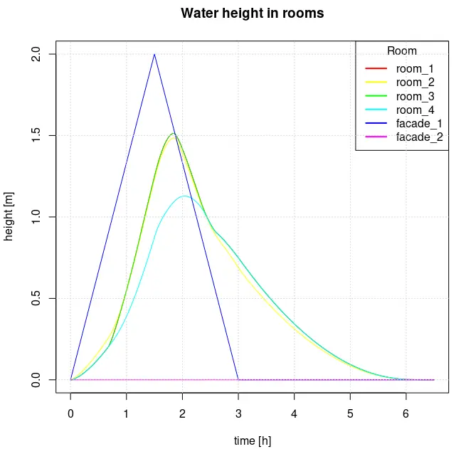
Multiple externals
If the dwelling is only flooded on one side or even if it is a terraced house you might need to define multiple exposed façades and external walls. The example below has an external wall exposed (wall_A) and the rest not exposed to floods. Note that we now provided two sets of facades for the parameters exposition and depth.
We can see that the water level is lower on average compared to the first exemple. Rooms further from the flooded side have an even lower water height.
hydraulics = analyse_hydraulic(
  model = model,
  limnigraph = flood,
  opening_scenario = "close",
  stage = c("hydraulic", "display")
)
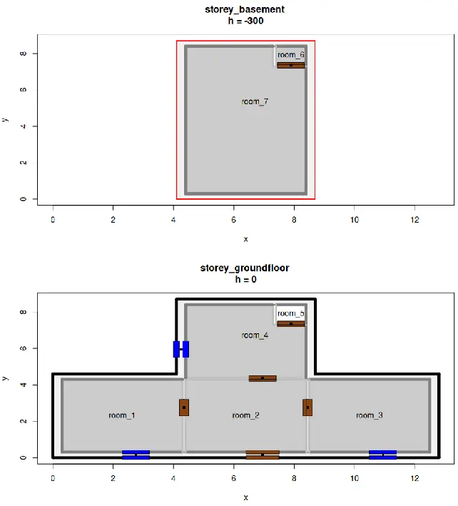
Multi level dwellings
The function analyse_hydraulic() can also be used to simulate hydraulic dynamics in multi-storey buildings, including those with basements. Let us show you how.
We will use now another shipped model: adu_t_basement. This model is almost the same as adu_t with a few additions: a basement under rooms 2 and 4 and a new room at the ground-floor level, at the back of the house, connecting this level with the basement.
As we did before, the first step is to call the function analyse_model() providing, at least, the values c("load", "extract", "hydraulic") to the parameter stage
model_basement = analyse_model(
  model = "adu_t_basement",
  type = "adu",
  stage = c("load", "extract", "hydraulic", "display"),
  path = model_path
)
A bigger building means more walls to take care of. Stay careful because multiple storeys generate multiple externals, and in floodam.building walls in different storeys can have the same name so it is important to locate precisely the exposed wall.
flood = generate_limnigraph(
  model = model_basement,
  time = c(0, 5400, 10800),
  depth = cbind(facade_1 = c(0, 1.5, 0)),
  exposition = list(
    facade_1 = list(external_groundfloor = c("wall_A", "wall_B", "wall_C", "wall_D", "wall_E", "wall_F",
      "wall_G", "wall_H"),
      external_basement = c("wall_A", "wall_B", "wall_C", "wall_D")))
)
Once your limnigraph is ready, you can call the function analyse_hydraulic() to compute the hydraulic dynamics of the building during your flood event.
hydraulic_basement = analyse_hydraulic(
  model = model_basement,
  limnigraph = flood,
  opening_scenario = "close",
  stage = c("hydraulic")
)
plot(hydraulic_basement, view = "level")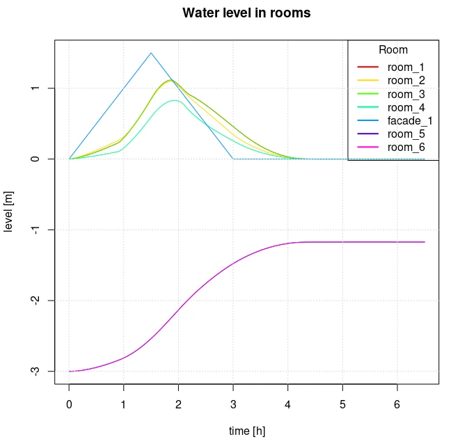
Go further
Congrats! you have made it through the tutorial! Now that you’ve mastered the basics, Let us see what you can do with all the functionalities of analyse_hydraulic() here.