Getting started
getting_started.Rmdfloodam.building produces flood damage functions for
built assets from a comprehensive inventory of those assets, covering
materials and components, the position in space (xyz) of those
components and the furnishing present (if any).
This vignette provides a high-level description of the overall
workflow you will use with floodam.building. The specifics
of some of the steps in this workflow are covered in separate
vignettes.
Basic workflow
The process starts by providing the input mentioned above. To make
things easier, floodam.building is shipped with various
testing models that include the specific inputs needed. The models are
available in your library’s installation folder, so just ask R to locate
them. You will also need to provide a folder where the output of
floodam.building can be stored (our example uses a
temporary directory):
#> Loading required package: floodam.building
library(floodam.building)
#> Python 3.8 detected: hydraulic tools available

#> set up model to use example shipped with floodam
model_path = list(
data = system.file("extdata", package = "floodam.building"),
output = tempdir()
)
Let us use the model called adu_t. This model proposes a
4-room house where three of them are organized around a central living
room. To generate a flood damage function for this model, we use the
function analyse_model() specifying load,
extract and damaging as analysis’ stages:
model = analyse_model(
  model = "adu_t",
  type = "adu",
  stage = c("load", "extract", "damaging"),
  path = model_path
)
#> Loading model 'adu_t'...
#>  - Structure of building.xml of 'adu_t' has been successfully checked
#>  ... successful
#> Extracting building information for 'adu_t'...
#>  - extracted:
#>          - parameter
#>          - storey
#>          - room
#>          - wall
#>          - opening
#>          - coating
#>  - missing (not found):
#>          - furniture
#>  ... Informations successfully extracted for 'adu_t'
#> Computing some values for 'adu_t'...
#>  ... Informations successfully extracted for 'adu_t'
#> Computing damage for 'adu_t'...
#>  ... Damaging successfully computed for 'adu_t'
#> End of analysis for 'adu_t'. Total elapsed time 2.66 secs
#> More information availabe at /tmp/Rtmp8GvIDa/model/adu/adu_t/adu_t.log
The function analyse_model() accepts input in both XML
and YAML formats. By default, the function looks for the XML format, so,
if you prefer to work with the YAML format, make sure that you specify
type_building = "yaml" when calling the function.
The output of the function analyse_model() is an object
of class model. This class of objects can be navigated like
nested R lists. Also, congratulations are in order! You have now
successfully processed your first model and have created your first
damage function. It is available inside the object model,
along with other information. Let us explore it further.
Basic visualization
floodam.building counts on methods to visualize key
information stored in model. For example, since
floodam.building uses highly detailed and spatialized
information of the dwelling, you can generate the dwelling plan.
#> visualization of the house's plan
plot(model, view = "top")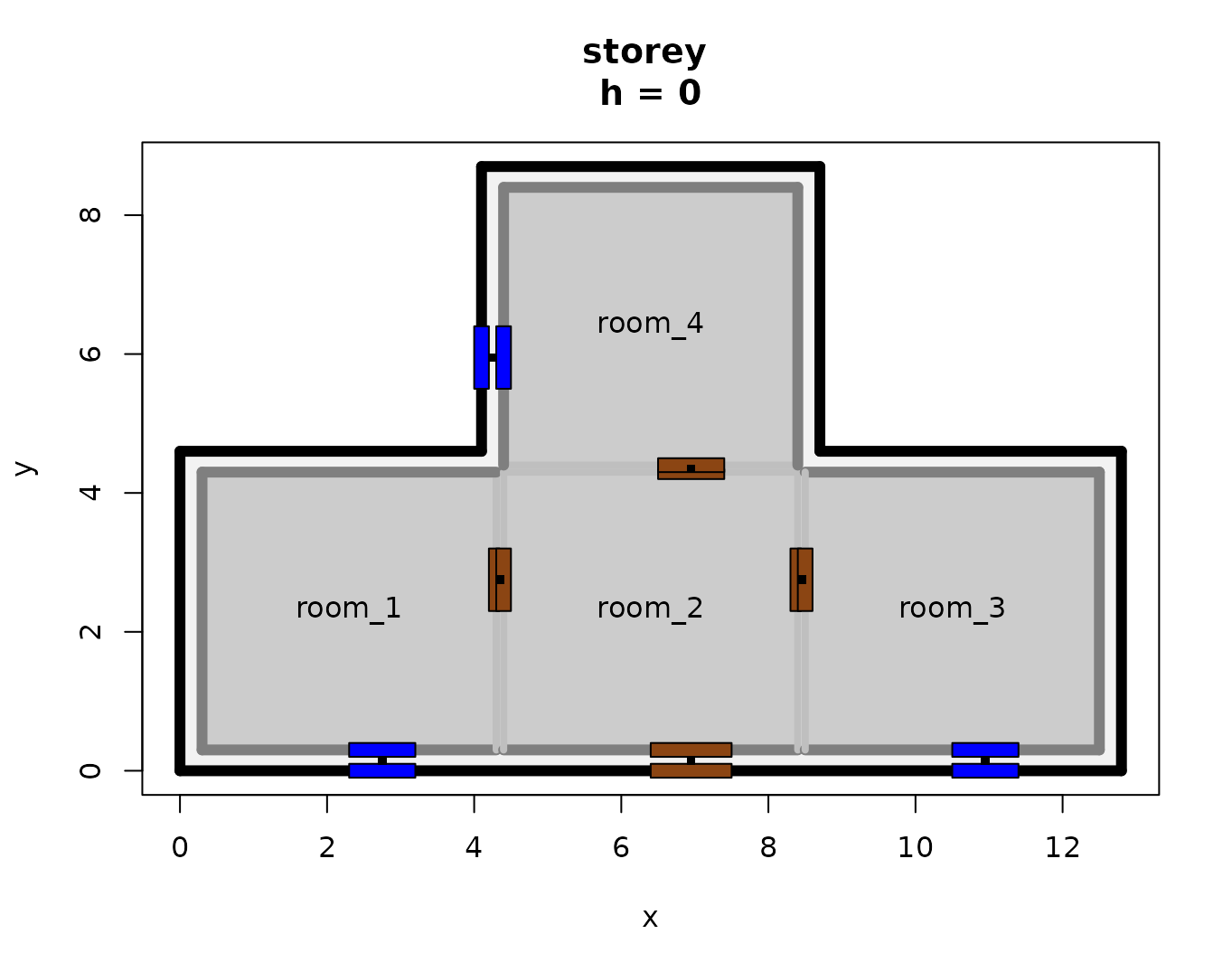
You also have available a default visualization of the damage
function estimated for this building. To generate it, simply change the
value of the parameter view.
#> visualization of the house's damage function
plot(model, view = "damaging")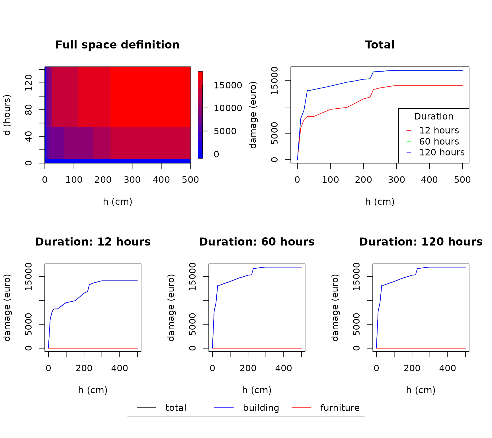
Now let us stop at this diagram for a moment to understand what you
are seeing. floodam.building calculates the damage
functions according to two different parameters: flood water depth and
flood duration. The bottom half of the figure contains three different
plots, each one presenting damage curves for flood events up to three
different durations: 12 hours, 60 hours and 120 hours. Any of these
plots also presents three different “curves”:
- Furniture: damage function corresponding to furniture only.
- Building: damage function corresponding to structural elements of the building only.
- Total: damage function aggregating both structural elements and furniture.
The top half of the figure contains two different plots. The top-right graph offers a comparison of the total damage curves for the three aforementioned flood durations. The top-left graph represents the amount of damage (in EUR) per flood depth (x-axis) and flood duration (y-axis).
Accessing data
The data to produce the plots above is stored within the object
model, in the slot damaging. Since objects of
class model can be navigated like nested lists, the information
is accessible via R’s standard operators for indexing operations.
Flood damage functions are stored as matrices. You will find several two main types of functions:
The absolute flood damage function, which expresses the damage in monetary units (EUR). It is located in the slot labelled absolute and available for the structural elements (building), for the furniture if any (furniture) and for the aggregation of both (total).
The surface flood damage function, which expresses the damage in monetary units (EUR) per unit of surface (squared meters). It is located in the slot labelled surface and available for the structural elements (building), for the furniture if any (furniture) and for the aggregation of both (total).
Let us check one of these matrices. In them, rows
represent the different flood depths for which
floodam.building calculates the damage (the default
resolution depth step is 10 cm) while columns represent
the maximum duration of the flood event. In this example, the damage
estimated for a 6-hour flood event with a flood depth of 40 cm is EUR
8211.42.
#> visualization of the house's damage function
head(model[["damaging"]][["absolute"]][["total"]], 10) |> knitr::kable()| 0 | 12 | 24 | 36 | 48 | 60 | 72 | 84 | 96 | 108 | 120 | 132 | 144 | |
|---|---|---|---|---|---|---|---|---|---|---|---|---|---|
| 0 | 0 | 0.000 | 0.000 | 0.000 | 0.000 | 0.00 | 0.00 | 0.00 | 0.00 | 0.00 | 0.00 | 0.00 | 0.00 |
| 10 | 0 | 6005.500 | 6005.500 | 6005.500 | 6005.500 | 7781.50 | 7781.50 | 7781.50 | 7781.50 | 7781.50 | 7781.50 | 7781.50 | 7781.50 |
| 20 | 0 | 7589.500 | 7589.500 | 7589.500 | 7589.500 | 9437.50 | 9437.50 | 9437.50 | 9437.50 | 9437.50 | 9437.50 | 9437.50 | 9437.50 |
| 30 | 0 | 8211.420 | 8211.420 | 8211.420 | 8211.420 | 13173.18 | 13173.18 | 13173.18 | 13173.18 | 13173.18 | 13173.18 | 13173.18 | 13173.18 |
| 40 | 0 | 8211.420 | 8211.420 | 8211.420 | 8211.420 | 13173.18 | 13173.18 | 13173.18 | 13173.18 | 13173.18 | 13173.18 | 13173.18 | 13173.18 |
| 50 | 0 | 8211.420 | 8211.420 | 8211.420 | 8211.420 | 13325.34 | 13325.34 | 13325.34 | 13325.34 | 13325.34 | 13325.34 | 13325.34 | 13325.34 |
| 60 | 0 | 8477.908 | 8477.908 | 8477.908 | 8477.908 | 13452.33 | 13452.33 | 13452.33 | 13452.33 | 13452.33 | 13452.33 | 13452.33 | 13452.33 |
| 70 | 0 | 8744.396 | 8744.396 | 8744.396 | 8744.396 | 13579.31 | 13579.31 | 13579.31 | 13579.31 | 13579.31 | 13579.31 | 13579.31 | 13579.31 |
| 80 | 0 | 9010.884 | 9010.884 | 9010.884 | 9010.884 | 13705.81 | 13705.81 | 13705.81 | 13705.81 | 13705.81 | 13705.81 | 13705.81 | 13705.81 |
| 90 | 0 | 9277.372 | 9277.372 | 9277.372 | 9277.372 | 13832.31 | 13832.31 | 13832.31 | 13832.31 | 13832.31 | 13832.31 | 13832.31 | 13832.31 |
Learn more
The rest of the vignettes provide more information on several different aspects. Please check:
- The structure of the input file of floodam.building and the From the architect’s plan to the input file of floodam.building vignettes to learn how to create your own input files.
- The Simulating the hydraulic behavior of the interior of a building vignette to learn how to simulate the internal hydraulic behavior of a building.